Article

How I Transformed Lab Efficiency with Process Engineering Tools

Work breakdown charts, network diagrams, and Python cut a 100-sample turnaround from months to weeks

Blaise Mibeck · Cubic Labs LLC · May 2025

Download PDF All articles and white papers

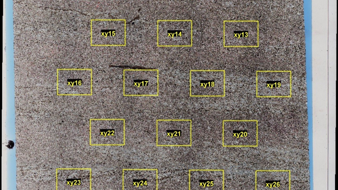
The challenge: analytical bottlenecks in a high-volume research lab

I used to work in a university lab that specialized in natural material analysis. It began receiving larger sample sets, 50 to 100 samples, with tighter deadlines. Sample requests from our subsurface research group often started with one analysis method and then grew to include the full suite: X-ray diffraction (XRD), X-ray fluorescence (XRF), optical microscopy, electron microscopy, and external micro-CT scanning.

The unpredictable workload caused real inefficiencies:

• Analysts did XRD phase identification without knowing the elemental composition, and often had to redo the work when that information arrived.
• Timelines, priorities, and responsibilities were unclear.
• Staff spent too much time on progress reporting and too little on sample preparation and analysis.

Management considered outsourcing the analytical work. Instead, my team and I redesigned the workflow using concepts from process engineering.

The solution: system analysis and process engineering

Step 1: Detailed process mapping and work breakdown

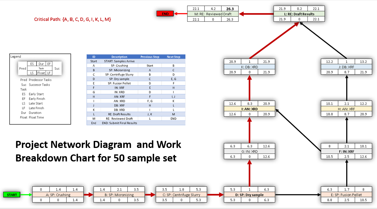
I treated the lab as a system. I discussed sample preparation and analysis with each lab member, and the discussions became a work breakdown chart that recorded:

• Material and time costs for each sample preparation and analysis type.
• Person-time versus machine-time requirements.
• Inputs and outputs for each step.
• Dependencies between analytical techniques.

The chart revealed opportunities for parallel work that were invisible when each process was viewed alone. When I found tutorials on project network diagrams, I felt I had discovered gold. Analyzing hundreds of samples with limited people and equipment resembles constructing a building or designing a circuit. It comes down to efficient use of resources and identifying the steps that, if delayed, delay the entire project.

Step 2: Designing an integrated analytical workflow

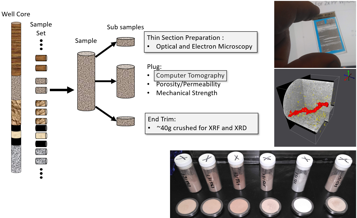
Rather than treating each request as a separate project, I developed a standard “analysis suite” that optimized sample handling:

1. Split a core plug into subsamples for thin section, CT, and XRF/XRD.
2. Send the thin-section and CT samples out.
3. Micronize the XRF/XRD subsample and split it into XRF and XRD samples.
4. Create fused beads for XRF.
5. Collect XRF and XRD results and combine them during XRD analysis.
6. Collect thin-section images and process the CT data.
7. Make all data available for internal review.

This removed redundant sample preparation and let analyses run in parallel. SEM-EDX was reserved for special cases such as element mapping and microstructure analysis. I also treated data storage as part of the system and kept metadata in a relational database.

Step 3: Automation and digital integration

Automation amplified the new workflow:

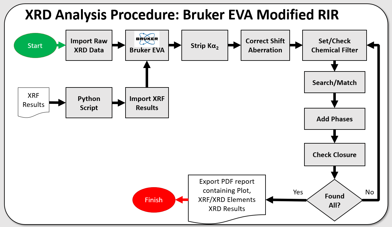
• Python scripts monitored the network drive and reported data availability in near real time.
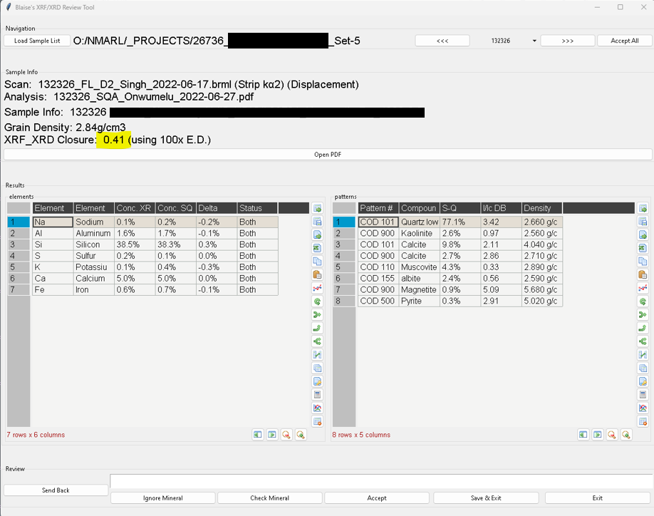
• Data organization tools prepared XRF results for XRD phase matching.
• Procedures filtered candidate mineral phases by elemental composition, which cut manual analysis time and made the work of several analysts more consistent.
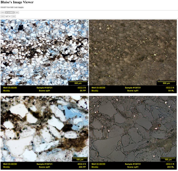
• Annotation of whole-slide microscopy images was automated, which produced an integrated visual database for geologists.
• Custom tools gathered information for review meetings, which made group data reviews more productive.

Step 4: Equipment selection

Equipment purchases followed the same logic. When I selected a new polarized light microscope, I chose objectives that removed the need for cover slips on thin sections. SEM analysis then needed no modification, which saved hours of preparation across large sample sets. In anticipation of the increased workload, our lab manager bought a bench-top Bruker D2 Phaser XRD with a very fast detector, which shortened scan times without losing data quality. Small details like these produced real efficiency gains.

The results

• Processing 100 samples went from months to weeks.
• Integration between analytical methods improved interpretation accuracy.
• Technicians spent less time on progress reporting and more time on analysis.
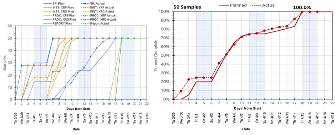
• Automated burn charts gave technicians and management a current view of project status.
• When equipment failed, we could calculate the effect on deadlines immediately and adjust.

Key lessons

1. Meet with the people doing the work. Start by learning what they do and what they need.
2. Communicate. Burn charts reduced stress and uncertainty for technicians and management.
3. Look at the whole workflow. Examining the entire process, not individual techniques, exposed inefficiencies that were invisible in isolation.
4. Standardize to scale. A core analytical suite let us handle more samples without a proportional rise in complexity.
5. Automate to extend what people can do. The Python scripts saved time and also allowed new ways of working and communicating across analytical methods.
6. Let the workflow guide equipment selection. Small decisions, such as microscope objectives or detector speed, affect overall efficiency.
7. Use project management tools in the laboratory. Work breakdown charts, project network diagrams, and burn charts are as useful in research as in construction.

With these principles, we turned a struggling laboratory workflow into an efficient one and kept our analytical services from being outsourced.